<< Go back to Posts
Warning : This document is still a draft

DARFT - Visual NLP Cheat Sheet.

In this post are described and illustrated common NLP models. The goal of this post is first to list the main models and then togive you the intuition behind it, without going deep into optimization problems.

Introduction

In this article, we provide simple illustration of the main technics used in NLP.

The technics are sorted by simplicity, from the oldest method to the most recent ones.

This article is not exhaustive, and its goal is not to list all exotic models, only the most relevant while trying to cover most NLP tasks. Nevertheless, we try to illustrate what is done in each and how they can be used for.

Table of Content

TODO

# Introduction
# ZIPFs Law
# Heaps or Herdan Law
# Stop-Words
# Tokenization
# Text Normalization - Stemming or Lemmatization
# Ngrams
# Huffman Trees
# Trees and Markov sentence Generation
# TFIDF
# TextRank
# RAKE - Rapid Automatic Key-phrase Extraction (2010)
# YAKE
# LSA - Latent Semantic Analysis
# pLSI - Probabilistic LSI
# LDA - Latent Dirichlet Allocation
# Markov Chain
# Hidden Markov Model
# Conditional Random Fields
# RNN: Recurrent Neural Network
# GRU
# LSTM: Long Short Term Memory
# BiLSTM
# Word2Vec
# Doc2Vec
# GloVe
# Seq2Seq
# VAE: Variational Auto Encoder
# BERT
# Attention
# Task
# Evaluation Metric
# Sources

Preliminaries

ZIPFs Law

Words are not distributed uniformly. There are words that are very frequent (the or is for instance), while many others do not occur frequently (e.g., schedule, saucepan). When studying the relationship between the word frequency and its rank, we observe that their relationship is described by a power-law:

\[\text{freq(word)} \propto \frac{1}{(\text{rank(word)} + \beta)^{\alpha}}\]

where $\alpha \approx 1$ in the case of a Zipf law. The coefficient is estimated to $\beta \approx 2.7$ in an Zipf-Mandelbrot law ($0$ in a regular Zipf law).

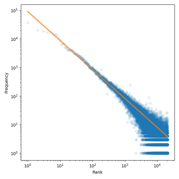
(Obtained from Stack Exchange biology tag corpus) Kaggle

Blue dots correspond to (word rank, word frequency) while the orange line corresponds to the Zipf law fit.

A power-law distribution is interesting because of its scale-free or fractal behavior: If a corpus of $n_0$ documents exhibit this behavior, then a subset $n_1 < n_0$ would also exhibit this same behavior.

Words are not the unique object following this kind of law ¹. Many other phenomena follow a power law distribution (graph degree, city size ², ³, passwords ⁴…). Power-law is the result of a process, not the explanation of why elements are distributed like that. Almost all language exhibit this Zipf law, with the same coefficient.

Heaps or Herdan Law

The number of distinct words $V$ in a corpus made of $N$ words are related by:

\[|V| = k N^{\beta}\]

where $\beta \in [0.67, 0.75]$

Stop-Words

When your goal is to categorize a text, to represent it with its main keywords, if you study frequency, top keywords would be words like:

is, the, there, they, want, where, whom, on, in, are, I, we, do, not,…

This is purely non-interesting. To ease the analysis of a text, these words are removed.

To avoid typing your own list, there are many available online on GitHub or elsewhere:

If removed, Part-of-speech tagging (for instance) cannot be done anymore because the sentence structure is degenerated.

Tokenization

Machine learning algorithm are unable to deal with “raw words” or raw ASCII characters. Instead, algorithms need word to be represented as a fixed-size identifier.

Tokenization can be replacing a word of arbitrary length by a number, or by a vector. For instance, if we have the two following sentences:

the dog is nice
the cat is cute

We have six unique words, and we can assign an ID to each of them:

{"the": 0, "dog": 1, "is": 2, "nice": 3, "cat": 4, "cute": 5}

The sentences are transformed into:

(0)-(1)-(2)-(3)
(0)-(4)-(2)-(5)

An equivalent way to represent these words is using binary vectors, where only one position is equal to one (the ID location), while all others are equal to zero.

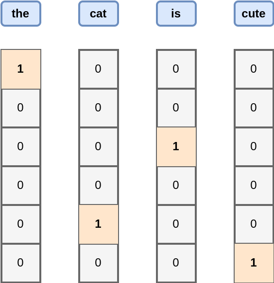
This vector form is very practical to make efficient computation on GPU for instance. If you want to compute the frequency of all words, you just need to add all binary vectors together. Each row would correspond to the number of occurrences.

This representation is very useful for neural networks.

Because these vectors are sparse, it is sometimes more convenient to represent them by their ID. For instance, for cute, represented by 5 = 101, we need three bits. To represent the full vector, we need 5 bits. Therefore, we need to be able to switch quickly of representation.

More advanced tokenization approaches

BPE: Byte Pair Encoding (Senrich, 2016)
WordPiece (Nakajima, 2012)
A new algorithm for data compression

Issues

Multi Word Expression: New York, San Francisco.
Abreviation: I'm = I am
Punctuation: Ph.D.
Prices
URL
Neologisms

NLP Standford

Text Normalization - Stemming or Lemmatization

From one word, we can derive many other words:

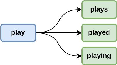
This is for verbs, but it applies to nouns (with -s for plural, -ment in entertainment, -ly in conditionally). When studying keywords or topics, we want to concentrate frequencies over one single term. With simple rules, we can remove the end of these words.

However, there are many irregular verbs in english, so we need to pay attention to them. Next, there are words ending with y, like summary which transforms into summaries.

Lemmatization is finding the root word. For instance, am, are, was, were, being, been are transformed into be

Stemming is cutting the end of the word to keep the root word. For instance, summary, summarizing, summaries, … are transformed into summar, even if this word does not exist in the dictionary.

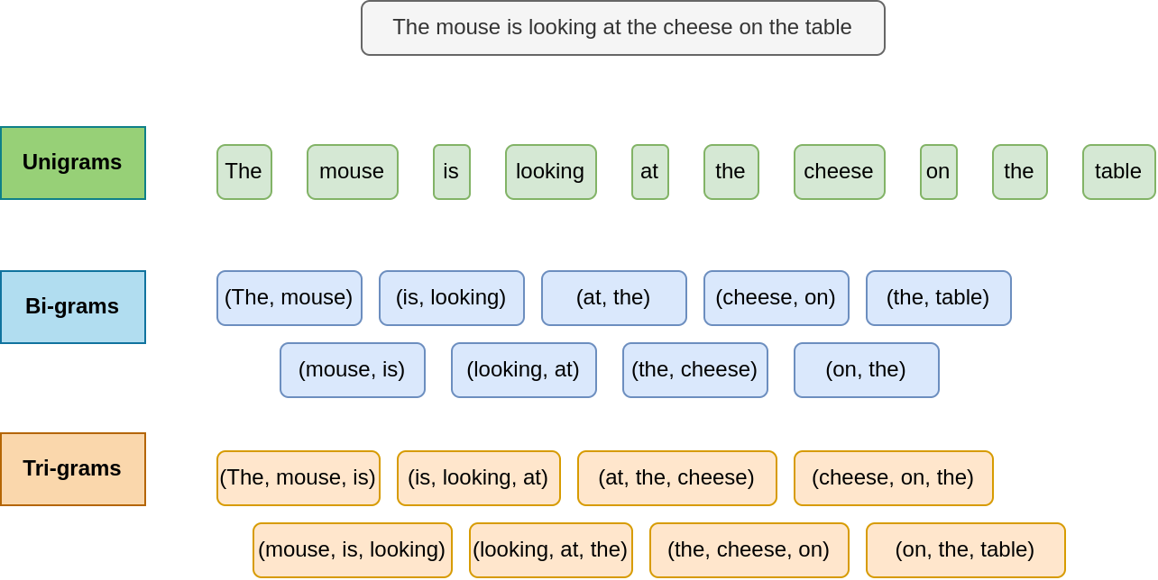
Ngrams

A n-gram is a sequence of n successive token. If a token is a word, a bi-gram is a two-words sequences, tri-gram, three successive words, etc. It is not relevant to study n-grams for large n, as the probability to see twice the same n-gram becomes relatively low.

Compared to single token, they are helpful to keep a little bit of context around a word or learn the grammar.

Generated with deep AI

To mark the beginning and the end of a sentence, we can add “starting” and “closing” tokens. This way, we can create sentence generators, where we feed the start token as input and wait for the closing one.

Huffman Trees

Huffman Trees help for data compression. If we have $n$ words, without optimization, we can represent a word using $\lceil\log_2(b)\rceil$ bits. Nevertheless, we can do better than that.

As discussed earlier, some words are more frequent than others. We can take advantage of the frequency to compress a message:

a frequent token receive a short binary code,
an infrequent token receive a longer binary code.

This way, on average, the number of exchanged bits is reduced.

Example

If we have the two sentences:

the cat is nice, with 15 letters
the dog is great, with 16 letters

we have 6 distinct words:

If we code token instead of letters, as we have 6 different words, we need 3 bits (which could encode 2^3 = 8 token). Because we have four words in each sentence, a sentence cost 3 x 4 = 12 bits, which is much better than 16 ASCII characters.

If we build a Huffman tree using these word frequencies:

{
  'is': 0.25,  'the': 0.25, 'great': 0.125,  'dog': 0.125,  'cat': 0.125, 'nice': 0.125}

We obtain the following tree:

is and the, the two most frequent words get a code of length 2, while the four others get a code of length 3.

Using Huffman codes, the two sentences are represented by the following binary strings:

10 (the) + 110 (dog) + 01 (is) + 111 (great) = 1011001111
10 (the) + 001 (cat) + 01 (is) + 000 (nice) = 1000101000

The reading is non-ambiguous: there is a single way to read the bitstring. However, we cannot start reading in the middle of the string (because code-words do not have the same length).

We summarize in this table the number of bits necessary to transmit the two sentences:

Sentence	ASCII	Simple Token	Huffman
I	`15 x 8 = 120 bits`	`4 x 3 = 12 bits`	`2 x 2 + 3 x 2 = 10 bits`
II	`16 x 8 = 128 bits`	`4 x 3 = 12 bits`	`2 x 2 + 3 x 2 = 10 bits`

Huffman is better than the simple naive token encoding. However, the improvement is relatively low. Nevertheless, over large text, the gains are much more important.

Huffman Trees are described in a previous article: Plainsight

Code to Create the Tree from Frequencies

def get_huffman_codes(freqs):
  """
  Compute the Huffman codes corresponding to the given word frequencies.

  :param freqs: a list of frequencies (non ordered)
  :rparam: the list of binary codes associated to each frequency
  """
  lst = sorted(map(lambda x: (x[1], [x[0]]), enumerate(freqs)))

  # Initialize code words
  dic_code = dict([(ID, '') for ID, _ in enumerate(lst)])

  while len(lst) > 1:
      # The first one has the lowest frequency, which would get a 1
      m1, m0 = lst[0], lst[1]

      # Iterate over all the IDs, and happend a 1 or a 0
      for c in m1[1]:
          dic_code[c] = "1" + dic_code[c]
      for c in m0[1]:
          dic_code[c] = "0" + dic_code[c]

      f_tot  = m1[0] + m0[0]
      ID_tot = m1[1] + m0[1] # List concatenation

      # For very large list of words, this is not optimal
      # It does the job for small inputs.
      lst = sorted([(f_tot, ID_tot)] + lst[2:])

  return list(dic_code.values())

The usage is the following:

dic_freqs = {'great': 0.125, 'is': 0.25, 'the': 0.25,  'dog': 0.125,  'cat': 0.125, 'nice': 0.125}
lst_codes = get_huffman_codes(dic_freqs.values())
dic_codes = dict([(word, code) for word, code in zip(dic_freqs.keys(), lst_codes)])

Usages

Huffman trees can be used at the letter level or at the word level. However, it can be used to represent any categorical object. It is not limited to text.

For short corpus, this might not be helpful, as we need to transmit (or store) how to read the binary string.

Markov Models

These models are not used anymore in NLP. However, there are good to know for other discipline or for making generators

Markov Chain

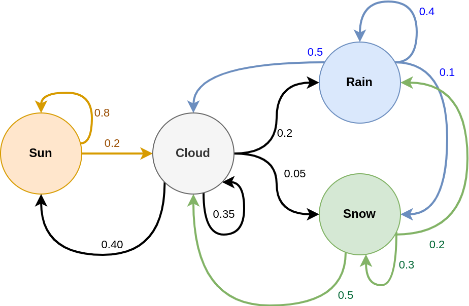
The Markov Chain is a simple generative model.

There is a finite set of state $W = [w_1, w_2, ..., w_s]$ which are the possible observable values. This model generates a sequence of random variables $X = (X_1, X_2, ..., X_T)$ where transition between one variable to the next one is fully explained by:

\[P(X_{t} = w_i | X_{t-1} = w_j)\]

Meaning that the choice for the next state fully depends on the current state.

In the above examples, W = [sun, rain, snow, cloud], and possible transitions (i.e., $P(X_t | X_{t-1}) > 0$) are materialized by arrows. Here, it is impossible to reach snow from sun. However, the snow state can be reached in two steps, by first jumping on the cloud state.

The probability to observe the states is not uniform. For instance, because the probability to move from cloud to snow or rain to snow are very low, we might not see the snow state that often.

Usage

There are two possible starting points:

you have a sequence of words, or
you have defined (or given) the MC diagram

Sequence of Word

In that case, you do not know $P(X_t| X_{t-1})$. You can find the the transition probabilities by looking at co-occurrences:

\[P_{i \rightarrow j} = P(X_t=w_j | X_{t-1} = w_i) = \frac{\#\{\text{"w_i w_j"}\}}{\#\{w_i\}}\]

I.e., the number of time the co-occurrence pattern w_i w_j occurs VS the w_i frequency.

Generating

Generating a sequence is super easy:

Initialization: Set $X_0$ by selecting a random state (or not) from $W$.

Iteration:

Pick a number uniformly at random $r \sim U(0, 1)$
Given this number, select the next state according to $P(X_t \rvert X_{t-1})$

Termination: Stop when the target number of elements is obtained or when another stopping condition is met.

Example using the above Diagram

import numpy as np

states = ["sun", "rain", "cloud", "snow"]
n_states = len(states)

# Transition matrix
T = np.array([
    [0.80,    0, 0.20, 0.  ],
    [0.,   0.40, 0.50, 0.10],
    [0.40, 0.35, 0.20, 0.05],
    [0.,   0.20, 0.50, 0.30]
])

# Sequence Generation
n_gen = 30 # Number of tokens to generate.

i_start = np.random.randint(n_states)
seq_i = [i_start]
for _ in range(n_gen):
    i_start = np.random.choice(n_states, p=T[i_start])
    seq_i.append(i_start)

# Convert to string the state ID
seq = list(map(lambda i: states[i], seq_i))
print(" - ".join(seq))

For a given trial, we obtained:

sun - sun - sun - sun - sun - cloud - rain - cloud - sun - cloud - sun - sun - cloud - rain - snow - rain - cloud - rain - cloud - cloud - sun - cloud - rain - rain - rain - cloud - snow - cloud - cloud - cloud - rain

To learn T from a sequence, we need:

Identify the number of token / n_states
Count the number of co-occurrence
Normalize the matrix

Here is the example while skipping the first step:

# Estimate the transition matrix
T_est = np.zeros((n_states, n_states))
for i, j in zip(seq_i[:-1], seq_i[1:]):
    T_est[i, j] += 1

# Normalize to get Sum_j P(X_j | X_i) = 1
T_est = (T_est.T / T_est.sum(axis=1)).T

T_est.round(2)

> array([[0.8 , 0.  , 0.2 , 0.  ],
       [0.  , 0.41, 0.59, 0.  ],
       [0.33, 0.3 , 0.23, 0.13],
       [0.  , 0.25, 0.75, 0.  ]])

As you can see, the transition probabilities estimated for the snow state are different from the initial model. Here, we learned over a sequence of 100 observations, which is insufficient. We would need a larger sequence to get something more accurate.

Practical Implementation

When dealing with a few state, a matrix works well. For a large corpus, the sparsity will increase. It is recommended to use a tree instead (or python dictionary) to stay efficient in terms of memory.

High Order MC

In the first-order Markov Chain, the transition exclusively depends on the previous state.

In the $k$-order version, the transition from the current state to the next one depend on the $k$ previous states:

\[P(X_t = w_i | X_{t-1}, ..., X_{t_k})\]

Rather than predicting a word with the previous one, you predict the word using the previous $n$-gram.

Caveat: When the order of the chain is too high, it is difficult to learn the conditional probability distribution, as we may have only one example per $n$-gram. This makes the model highly deterministic and unusable.

Object

The Markov chain considers a finite set of states $W$. In practice, it can be:

Words
Letters
Token (sub-words)
Grammatical class
Other categorical variables.

Example with NLTK + markovify Markov Chain (not HMM) for text generation

Hidden Markov Model

A tutorial on Hidden Markov Model, 1989. ⁵

A HMM is an extension of the Markov Chain model. The only difference is that states are hidden. However, what we observe depend on the current state.

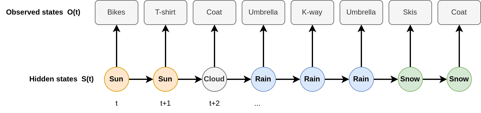
Here, we reuse our previous example with weather. Suppose you are in an office with no window. You would like to know, given how your colleagues are dressed (the observed values), what is the weather outside (the hidden states).

In NLP, HMM are useful for learning grammar. You know that there are rules such as Noun + Verb and Verb + Attribute. We know them because we learned them. However, instead of writing them down by hand, we can ask the model to learn these rules and to classify words into these categories.

Probability Model

About Observations

The observation $O_t$ only depends on the current state $S_t$:

\[P(O_t | S_t)\]

An observation $O$ can be observed while in different states. I.e., $P(S | O) \neq 1$: we cannot identify deterministically the state given the observation (sometimes we can, but most of the time, we cannot).

Observations can be categorical (i.e., we have a finite set of non-ordered values) or discrete / continuous. In the later case, we need to discover the parameters of the generating models for each state.

About States

The transition probability from one state $S_t$ to another depends on the previous one:

\[P(S_t | S_{t-1})\]

Same as for Markov Chains, high-order HMMs exist, where the transition to the next state depends on the $k$ previous ones:

\[P(S_t | S_{t-1}, S_{t-2}, ..., S_{t-k})\]

Fitting the Model

The parameter of the HMM are trained thanks to the Viterbi algorithm. This is a kind of Expectation-Maximization algorithm. The only thing we need to set by hand is the number of desired states.

Slides Introduction

Paper Standford What is HMM ?

Keyword Extraction

TFIDF

Term Frequency - Inverse Document Frequency (1983) ⁶

Idea

The name of this method is exactly what we need to compute.

A word in a document is scored thanks to two quantities:

the word frequency within the current document,
the word document frequency within the whole corpus, which is the number of documents containing at least on occurrence of this word.

The largest the word frequency the better. However, if a word is present in all documents, it might be a common word, therefore less interesting than a word which occurs in a few documents.

Use-Cases

TF-IDF can help to:

identify common words
identify uncommon words
score documents

Processing

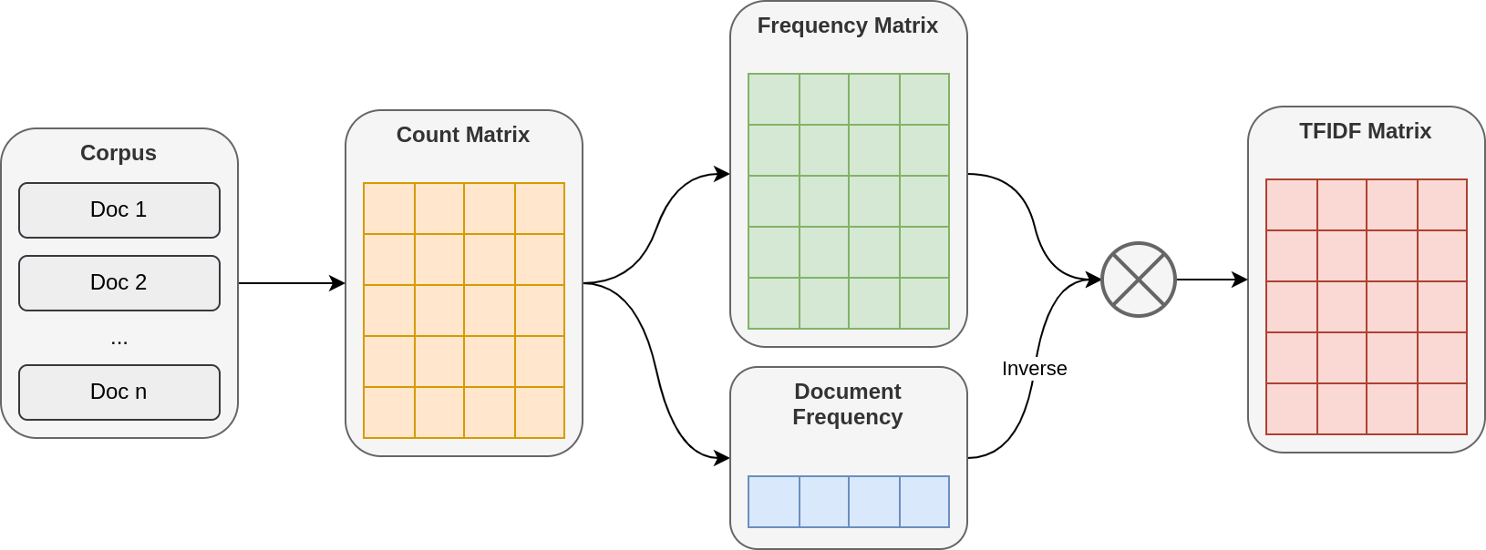
Suppose you have a corpus $\mathcal{D} = \{D_1, D_2, ..., D_n\}$ made of $n$ documents. There are $k$ unique words $\mathcal{W} = \{w_1, w_2, ..., w_k\}$.

From that, we can create a count matrix $X$ where:

\[X_{i, j} = \#\{w == w_j\}_{w \in D_i}\]

From this count matrix, we can extract two things:

The Term Frequency matrix
The Document Frequency array, which is the number of documents containing a given word.

which are defined as:

\[TF_{ij} = \frac{X_{i, j}}{\sum_{\ell=1}^k X_{i, \ell}}\] \[DF_j = \#\{w_j \in D\}_{D \in \mathcal{D}}\]

The idea of TFIDF is that when a word occurs frequently in a dataset, than it counts less that a word which is only present in a few document. Therefore, the document frequency $DF$ is transformed into the inverse document frequency $IDF$ defined as:

\[IDF_j = \frac{n}{DF_j}\]

The final TF-IDF matrix is simply:

\[TF-IDF = TF \times IDF_j\]

where the larger the score, the better.

Usages

Sort words of document i in decreasing order:

order_word = np.argsort(-TFIDF[i])

Sort documents based on their novelty (compared to the corpus):

order_doc = np.argsort(-TFIDF.sum(axis=1))

Variants

There exist a few variants of TFIDF ⁶, based on how the term frequency and inverse document frequency are computed. These variants are here to address cases when documents are very long (therefore, all words occur in almost all documents, despite their low frequency. In that case, the DF is very similar for all words), or when the document size is non-homogeneous.

TextRank

2004

Page Rank adapted to text.

PageRank was designed to identify “best web pages” using hyperlinks between pages. The idea of this algorithms is:

with a probability $(1 -d)$, jump on any node of the web graph
with a probability $d$, follow an hyperlink selected at random. If a node has $3$ hyperlink, then there is 1/3 chance to go on the first link.

At the start, each node has the same score $S(i) = 1$ Given the two rules, the algorithm update the scores until there is no more changes:

\[S(j) = (1 - d) + d \times_{i \in \mathcal{N}_j^{\text{parent}}}^n \frac{1}{|\mathcal{N}_i^{\text{children}}|} S(i)\]

A link is necessarily unweighted as a page is a page and occurs only once, so a link in has no weight. For text, a sequence can occur multiple times in a corpus. Therefore, TextRank takes co-occurrence frequencies into account.

If $w_{i, j}$ is the co-occurrence of the bigram $(i, j)$,

\[S(j) = (1 - d) + d \times_{i=1}^n \frac{w_{i, j}}{\sum_{\ell=1}^n w_{i, \ell}} S(i)\]

TODO example / Illustration

Co-occurrence windows of size 2-10 Evaluate single keywords. For multiple keywords, postprocessing phase. 20-30 iteration. Remove links with less than 0.0001 Keep top T vertices

Can be used for sentence extraction:

\[Sim(S_1, S_2) = \frac{|S_1 \cup S_2|}{\log(|S_1|) + \log(|S_2|)}\]

Cosine ? Possibility

Original Paper

In the same family:

RAKE - Rapid Automatic Key-phrase Extraction (2010)

RAKE aims to identify and rank keywords or set of keywords.

A text is pre-process by splitting elements where stop-words or ponctuation occur. We obtain isolated or grouped keywords.

TODO: EXAMPLE Example: initial text

This paper presents an unsupervised approach for keyword extraction from a document. Summarizing a research paper is not an easy task, it is time-consuming. For making summarization of documents much easier keywords are used. Keyword helps in summarizing a large amount of textual data. Keyword extraction is a process in which a set of words are selected that gives the context of the whole document. Here, we are proposing a graph-based model approach for extracting keywords from a research paper. The proposing method is a combination of Rapid Automatic Keyword Extraction (RAKE) algorithm and Keyword Extraction using Collective Node Weight (KECNW), in which candidate keywords are extracted using RAKE algorithm and selection of keywords using KECNW model. The final output of this methods are keywords extracted from a document with their rank

After the first segmentation based on punctuation and common stop-words, we get:

paper present — unsupervised approach — keyword extraction — document — summarizing — research paper — easy task — time-consuming — summarization — document — keyword — used — keyword help — summarizing — large amount — textual data — keyword extraction — proces — set — word — selected — context — document — proposing — graph-based model approach — extracting keyword — research paper — proposing method — combination — rapid automatic keyword extraction — rake — algorithm — keyword extraction — collective node weight — kecnw — candidate keyword — extracted — rake algorithm — selection — keyword — kecnw model — final output — method — keyword extracted — document — rank

Next, for each keyword, we measure:

its frequency, i.e., the number of occurrences
its degree, i.e., the number of keywords it appears with (the keyword itself is counted, therefore the minimal degree is one)

Then, a keyword receive a score: $\frac{freq(w)}{deg(w)}$.

	Freq	Deg	Score
rapid	1	4	4
automatic	1	4	4
node	1	3	3
weight	1	3	3
graph-based	1	3	3
collective	1	3	3
data	1	2	2
present	1	2	2
extracting	1	2	2
output	1	2	2
unsupervised	1	2	2
task	1	2	2
approach	2	4	2
time-consuming	1	1	1
proces	1	1	1
extraction	4	4	1
…	…	…	…
word	1	1	1
keyword	10	8	0.8
summarizing	2	1	0.5
document	4	1	0.25

Individual keyword does not help that much to understand the content.

The final score of a group of keywords is the sum of word scores. For instance, rapid automatic keyword extraction is equal to:

4 (rapid) + 4 (automatic) + 0.8 (keyword) + 1 (extraction) = 9.7

Therefore, the top key-phrases are:

9.8 rapid automatic keyword extraction
9.0 collective node weight
7.0 graph-based model approach
4.0 unsupervised approach
4.0 textual data
4.0 large amount
4.0 final output
4.0 easy task
3.0 paper present
…

The three top one are very good candidate from my human perspective. The bottom ones are not that much interesting.

Slides

Dedicated Chapter

YAKE

Link

BM25

TODO: TFIDF but more advanced.

Topic Modeling

LSA - Latent Semantic Analysis

Or LSI for Indexing, (1990).

Idea

LSA is the first method to introduce topics. Indeed, previous recommender system or search algorithms would compare a query to documents. If a query contains the term animal, many documents talking about cat or dog would also have the term animal in. However, not all. Some documents containing cat will have zero occurrence of the terms animal. Here comes the topic idea: LSA will learn which words are similar and appears in the same topic. This way, even we do not explicitly the term animal, related documents will match.

Method

LSA exploits the SVD eigenvector decomposition technic.

As a reminder, Singular Value Decomposition allows to get $U$, $V$ and $\Sigma$ verifying:

\[X = U \Sigma V^T\]

Where $\Sigma$ is a diagonal matrix.

This way, the method identify “topics”, where their strength is represented by its eigenvalue in $\Sigma$.

$U_i$ (a row of $U$) represents the weight attributed to each topic for document $D_i$, while $V_j$ represents the weight of words $w_j$, i.e., the context where the word appears.

SVD is a general eigenvalue decomposition matrix. In LSA, for the aim of identifying topics, it is recommended to decompose the TF-IDF matrix. This way, words are already weighted by their relevance.

EXX

Deerwester, S., Dumais, S.T., Furnas, G.W., Landauer, T.K. and Harshman, R. (1990), Indexing by latent semantic analysis.

Illustration of Singular Value Decomposition

In the illustration, the different shade of colors are only here to materialize the features / elements belonging to a given topic. Nevertheless, unless for $\Sigma$ where eigenvalues are sorted by decreasing order. Topic vectors are orthonormal, i.e., $U^T U = Id$ (ortho: $U_i^T U_j = 0 | i \neq j$, normal: $U_i^T U_i = 1$), both for $U$ and $V$.

Usage

The main usage of LSA is three-fold:

Rank topics by dominance using eigen-values $\Sigma$
Rank / group documents per topic using $U$
Identify topic vocabulary using $V$

LSA can be used for document clustering (or word clustering) using the first eigenvectors.

It can be used for efficient documents (words) comparison as not all eigenvectors are useful (low weights eigenvectors can be discarded without impacting the outcome).

It can be used for document compression.

U, S, V = np.linalg.svd(TFIDF)

k = 10 # Number of topic left
TFIDF_compress = (U[:,:k] * S[: k]) @ V[:k]

Comparing two Documents

A document is represented by a row of $X$. To compare document $i$ and document $j$, we need to make their product $\mathbf{x}_i^T \mathbf{x}_j$, as in the cosine similarity (well, this only hold if SVD is done on the term-frequency matrix where rows sum to 1, not the TFIDF one).

If we use the matrices obtained from SVD, $\mathbf{x}_i^T = (\mathbf{u}_i \Sigma V^T)^T$. Therefore, $Sim(i, j) = (\mathbf{u}_i \Sigma V^T) (\mathbf{u}_j \Sigma V^T)^T = \mathbf{u}_i^T \Sigma^2 \mathbf{u}_j$

We can speedup the comparison by keeping the $k$ first topics, using $\hat{X}$

How to Represent a Query ?

Matrices $(U, \Sigma, V)$ are obtained thanks to a corpus of $D$ documents. If we receive a query or a new document, we would like to transform it in the $U$ space, so we can compare this query to existing documents (or two queries together).

If $x_{new}$ is the vector representation of the unseen document, we want to find its representation in $U$, the topic-document space:

\[x_{new}^T = u_{new}^T \Sigma V^T\]

By multiplying both right sides by $V\Sigma^{-1}$, we obtain:

\[u_{new} = x_{new}^T V \Sigma^{-1}\]

(as $V^T V = Id$)

TODO: how to compare two elements. Need to look at the course on feature reduction

pLSI - Probabilistic LSI

While LSA/LSI are exact maths, where the document-word matrix is decomposed into eigenvalues and eigenvectors, pLSI provides the equivalent formulation in probabilistic terms.

$U_{i, j} = P(d_i | z_j)$ $\Sigma_{i, i} = P(z_i)$ $V_{i, j} = P(w_i | z_j)$

Because of their probabilistic distribution, we do not have relationships such as $U^T U = Id$. Instead, we have:

\[\sum_{i=1}^K \Sigma_i = 1\] \[\sum_{j=1}^K U_{i, j} = 1\] \[\sum_{j=1}^K V_{i, j} = 1\]

In this model, we assume that $d$ and $w$ are conditionally independent:

\[P(d, w | z) = P(d | z) P(w | z)\]

Therefore, $U \Sigma V^T = [P(d_i, w_j)]_{i=1:N,j=1:W}$. A document is a mixture of topics, and the observed words depend on these topics.

Graphical Representation

Parameter Estimation

The parameters are learned using the expectation-maximization (EM) algorithm:

During the $E$ step, we compute the expected posterior probability of $z$ given words and documents $P(z ; w, d)$
During the $M$ step, we update the parameters $P(w \| z), P(d \| z)$ and $P(z)$ using $P(z; w, d)$

Generative

pLSI is a generative algorithm. When parameters are obtained, it is easy to generate natural-looking documents.

Pick a document $P(d)$
Pick a class $P(z; d)$
Generate a word $P(w; z)$

Hofmann, Thomas. (1999). Probabilistic Latent Semantic Indexing.

Probabilistic Latent Semantic Analysis Dan Oneat¸˘aExplained

LDA - Latent Dirichlet Allocation

(2003)

LDA follows an intuition close to LSA, and can be seen as a more advanced version of pLSI:

We do not look at text structure, only words’ frequency.
We assume that words can be grouped into topics, and a word can belong to multiple topic at a time.
This is a generative algorithm (as pLSI).

Compared to pLSI where $P(z ; d)$ and $P(w ; z)$ are unconstrained, here we assume that both follow a Dirichlet distribution.

We have a corpus with $D$ documents, a vocabulary set with $W$ distinct words, and $K$ topics.

If we consider one topic:

The word distribution within a topic is $\pmb{\beta} \sim \text{Dirichlet}(\eta)$. I.e., if we know the topic, we know the probability of observing a given word.
In other words, $\pmb{\beta} = [\beta_i]_{i=1:W} = [P(\text{word} = w_i \| \text{topic})]$

If we consider one document:

A document is not about a single topic, it is a mixture of topics.
The topic proportion is $\pmb{\theta} \sim \text{Dirichlet}(\alpha)$
I.e., $\pmb{\theta} = [\theta_i]_{i=1:K} = [P(z_i \| d)]_{i=1:K}$
Two documents do not necessarily have the same topic distribution. If $\theta_1 \sim \text{Dirichlet}(\alpha)$ and $\theta_2 \sim \text{Dirichlet}(\alpha)$, it does not imply that $\theta_1 = \theta_2$

If we consider one word of a specific document:

an observed word belongs to a single topic at a time (i.e., the current location is not a mixture of topics).
we cannot say anything about successive words ($w_i$ can belong to topic n°1 while $w_{i+1}$ can belong to topic n°4)

Graphical Representation

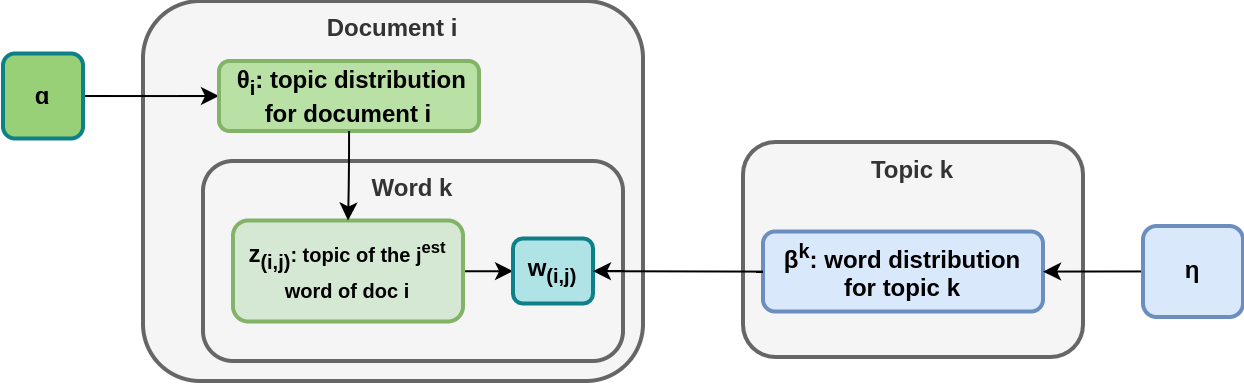
In this algorithm, there are two Dirichlet distribution with two distinct parameters:

$\alpha$ for documents’ topic distribution
$\eta$ for topics’ keywords distribution

A document $d$ is composed of a mixture of topics with proportion $\theta_d$, where $\theta_d \sim D(\alpha)$.

\[P(\text{topic} = k | d) = \theta_{d, k}\]

A topic $k$ is composed of a mixture of words with proportion $\beta_k$, where $\beta_k \sim D(\eta)$.

\[P(\text{word} = w_i | k) = \beta_{k, w_i}\]

During training, the algorithm need to learn $\alpha, \eta$ and determine $\theta$ for all words and $\beta$ for all topics. This can be done using the Expectation-Maximization algorithm.

Generative VS Discriminative

Despite its ability to “classify” words from a document into topics, LDA is a generative algorithm.

The difference between generative and discriminative algorithms is often difficult to grasp, as both are able to identify a word’s topic.

A discriminative model tries to learn the mapping $\text{word} \rightarrow \text{topic}$, i.e, a complex input mapped into a small concept space.
A generative model tried to learn the inverse mapping, $\text{topic} \rightarrow \text{word}$, i.e., a simple concept is expanded into a complex one.

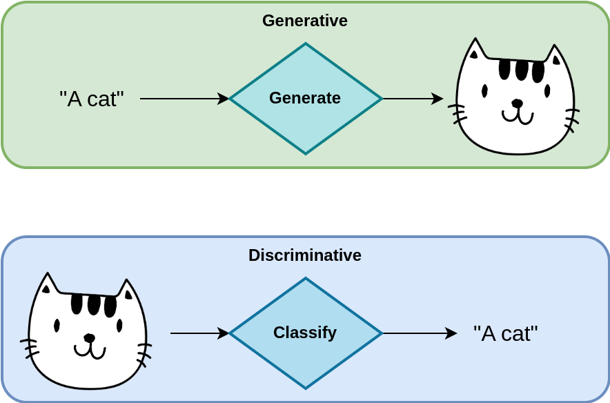
The issue in understanding generative algorithms is in their training.

In the case of supervised learning:
- discriminative algorithms are trained on (image, concept) pairs,
- generative algorithm are trained on (concept, image) pairs
In the case of unsupervised learning,
- the discriminative algorithm is trained with (image, ?), i.e., we do not provide concepts, they need to be learned.
- the generative algorithm is trained with (?, image), i.e., we do not provide concepts either. We cannot train a generative algorithm on (concept, ?), because it is possible to reduce the dimension of a space by learning similarities, however, it is not possible to expand the space without help.

Generating New Documents

When parameters are obtained, LDA can help to generate documents and their words. For that, the process is quite simple:

Generate $\theta \sim D(\alpha)$
Generate $N \sim \text{Poisson}()$ the number of words to generate
For each word:
- Generate the topic $z \sim Multi(\theta)$
- Generate the word $w \sim Multi(\beta^z)$

As said earlier, this algorithm does not pay attention to word order, only to frequency. To order words in a logical order, we need other algorithm. Therefore, most of the time, LDA is only used to identify the hidden topics, not really to generate documents (adding more to the confusion between generative and discriminative models)

Additional Ressources

Conditional Random Fields

CRF

TLDR Paper: CRF for relational learning Paper: An intro, 2011 Slides

Discriminative While HMM Generative.

HMM:

\[P(y, x) = \prod_{t=1}^T P(x_t | y_t) P(y_t | y_{t-1})\]

$y$: State. Only depend on the previous one
$x$: Observation. Only depend on the current state.

Linear chain CRF: Bidirectionalily

\[P(y | x) = \frac{1}{Z(x)}\prod_{m=1}^M \exp(\lambda_m f_m(y_n, y_{n-1}, \mathbf{x}_n))\]

$Z$: Normalization constant.

Neural Networks

RNN: Recurrent Neural Network

Fundamental of RNN and LSTM Understanding LSTM, a tutorial Book RNN for prediction Slides Chapter color short

A Recurrent Neural Network can be seen as the generalization of the hidden markov model to continuous states. From one observation to another, the network keep in memory a real-value vector $\mathbf{h}_t$ which keep the information about the current state.

\[h(t) = tanh(W^{hx} x(t) + W^{hh}h(t-1) + b^h)\]

Applications

There are three common application for RNN:

Predict the next word in a sentence
Given a starting point, generate a full sentence
Translation: given a sentence, predict the converted sentence.

Generating text with RNN

Applications

GRU

LSTM: Long Short Term Memory

An LSTM is very similar to an RNN. The only conceptual difference is that the RNN keeps one state vector, while the LSTM keep two state vectors: one where the aim is to keep short term information while the second long term info..

BiLSTM

Word2Vec

“Efficient Estimation of Word Representations in Vector Space (2013) ⁷

Word2Vec is a simple yet effective two-layers fully-connected neural network used to predict words given context.

Network Architecture

One-hot encoded vectors are fed to the network.

The first layer aims to embed the word (or token) in a small dimensional space and switch the representation from binary to continuous. The binary vector of size $N$ is transformed into a real-valued vector of size $V$ with $V < N$.

The second layer aims to project back a vector from the latent space to the word space in order to predict the next word. This layer is made of $N$ softmax units ($\frac{e^x}{\sum_i e^{x_i}}$).

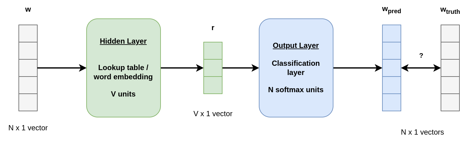
To train the model, we compare the generated vector $\mathbf{w}_{pred}$ to the actual binary vector $\mathbf{w}_{truth}$ and backpropagate the errors to update the weigths.

Prediction Strategies

Word2Vec covers two predictions strategies:

Continuous Bag of Words (CBoW): Given the context / several words, the model tries to predict the missing/next word;
Skip Grams (SG): Given a single word, the model tries to predict the surrounding context words.

Continuous Bag of Words

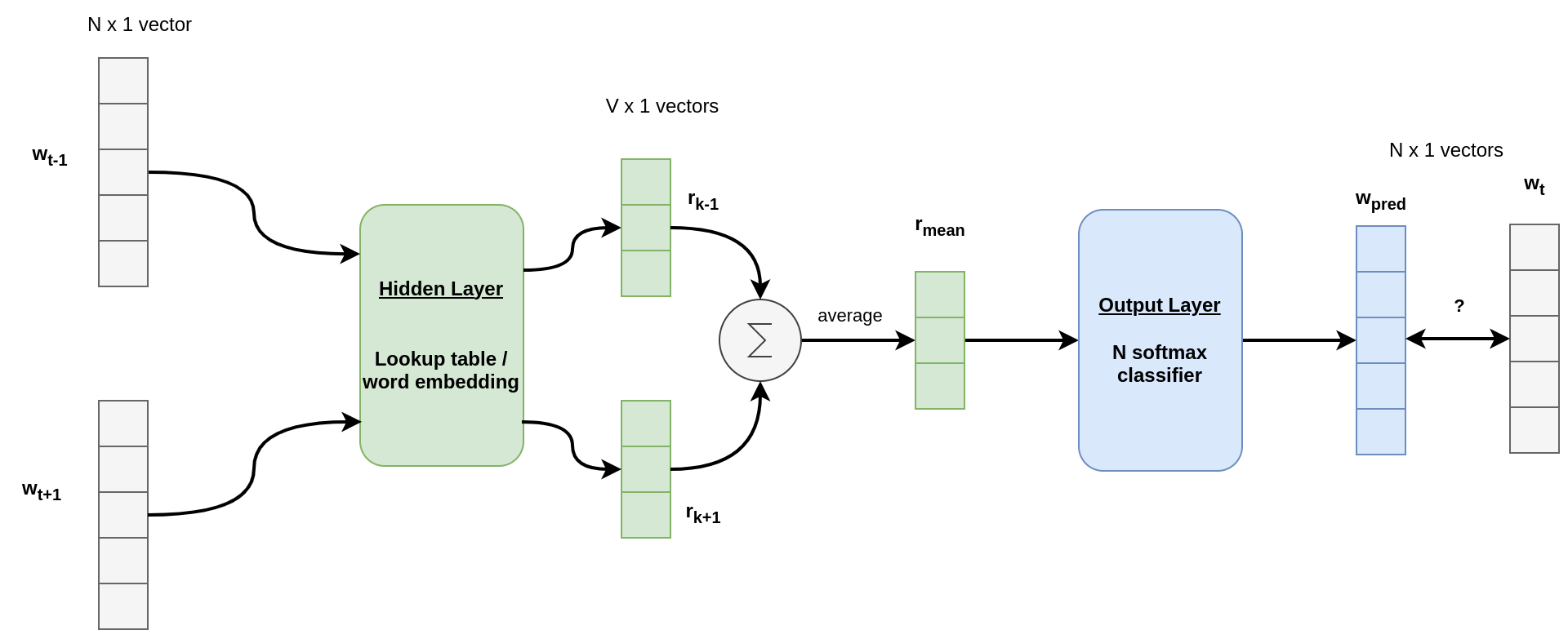
Here, the goal is to predict a missing word given its surrounding context. There are multiple definition of the task:

Next word prediction: Given w(t-k), w(t-k+1), ..., w(t-1) predict w(t),
Missing word prediction: Given w(t-k), ..., w(t-1), w(t+1), w(t+k) predict w(t).

In this task, we feed the network with several words (one at a time, the size of the layers are unchanged, and word order does not matter) to predict a single word.

For each of these words, the first layer provides their low dimensional representation. The vectors are averaged into a single vector $\mathbf{r}_{mean}$. This vector is the context representation in the low dimensional space.

$\mathbf{r}_{mean}$ is sent to the softmax layer which transforms it back to the word space.

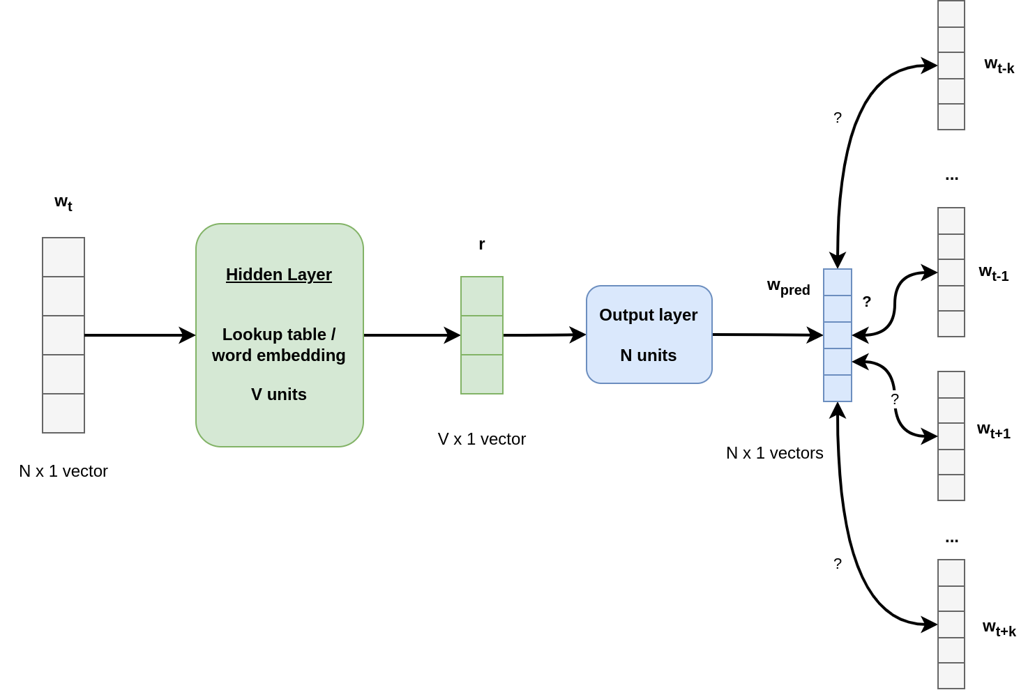
Skip Grams

While CBoW try to predict a single word using multiple input words, Skip-Grams does the opposite: Given a single words w(t), it tries to predict words within a context window of size $k$:

Symmetric case: w(t-k), ..., w(t-1), w(t+1), w(t+k)
Asymmetric case: w(t-k), w(t-k+1), ..., w(t-1) or w(t+1), w(t+2), ..., w(t+k)

It is important to note that Skip-Grams does not predict the word orders / or the word at position t+k. It only returns words that are likely to occurs within the context window.

As before, the hidden layer converts the binary token vector into a low-dimensional continuous representation.

The output layer is still a softmax layer, which provides words probabilities. By ranking them, we can list the most likely context words.

During training, we feed the network with w(t), and then compare it to the $k$ previous and the $k$ futures words.

Skip-Grams takes more time to train:

In CBOW, ([w(t-k) ..., w(t-1), w(t+1), ..., w(t+k)], w(t)) corresponds to a single training sample.
In SkipGrams (w(t), w(t-k)), …, (w(t), w(t-1)), (w(t), w(t+1)), (w(t), w(t+k)) are all training examples with input (w(t)) (there are exactly 2k training examples per window). This explains why SG is longer to train.

Doc2Vec

Distributed Representations of Sentences and Documents (2014) ⁸, ⁹

Doc2Vec follows the same intuition as Word2Vec. The difference is that they introduced a “paragraph ID” to keep memory of the overall context of the document.

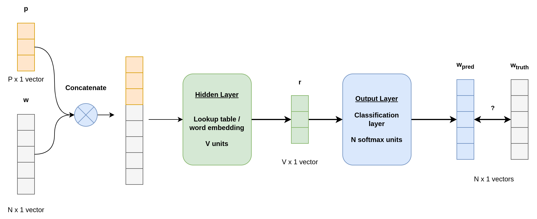
Two methods are introduced, which are analog to the one described in Word2Vec:

Paragraph Vector - Distributed Bag of words (PV-DBOW): This one is analogous to the Word2Vec Skip-gram. While skip-gram tries to predict elements in a context window thanks to a given word, PV-DBOW tries to predict the same elements while replacing the info-word by the paragraph identifier.
Paragraph Vector - Distributed Memory (PV-DM): This one is analogous to the Bag of Words model, where the paragraph vector is concatenated to the binary word vectors.

PV-DM

This model is similar to the Word2Vec-CBOW approach, where we use context to predict the missing word, plus the paragraph ID, which enable the network to memorize the main context of the current document.

For instance, if you have the sentence with a missing word: it was a very cute and lovely ???? which was crossing the street. From the previous words, it is impossible, without context, to know what ???? is.

If the document is about cats, then cat is a good candidate for ???
If the document is about dogs, then dog is a good candidate for ???
If the document is about cars, then car is a good candidate for ???

There are two possible architectures: word concatenation or word averaging.

Concatenation

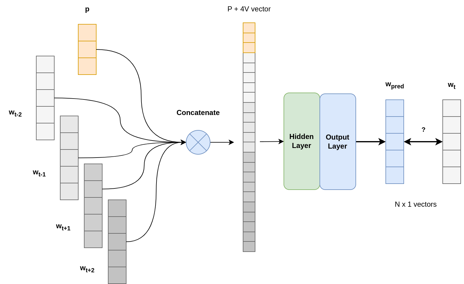
In that case, the context windows takes a fixed number of words to predict the missing one. Here, because of the vector size, the hidden layer has larger weights, therefore it takes more time to train.

Averaging

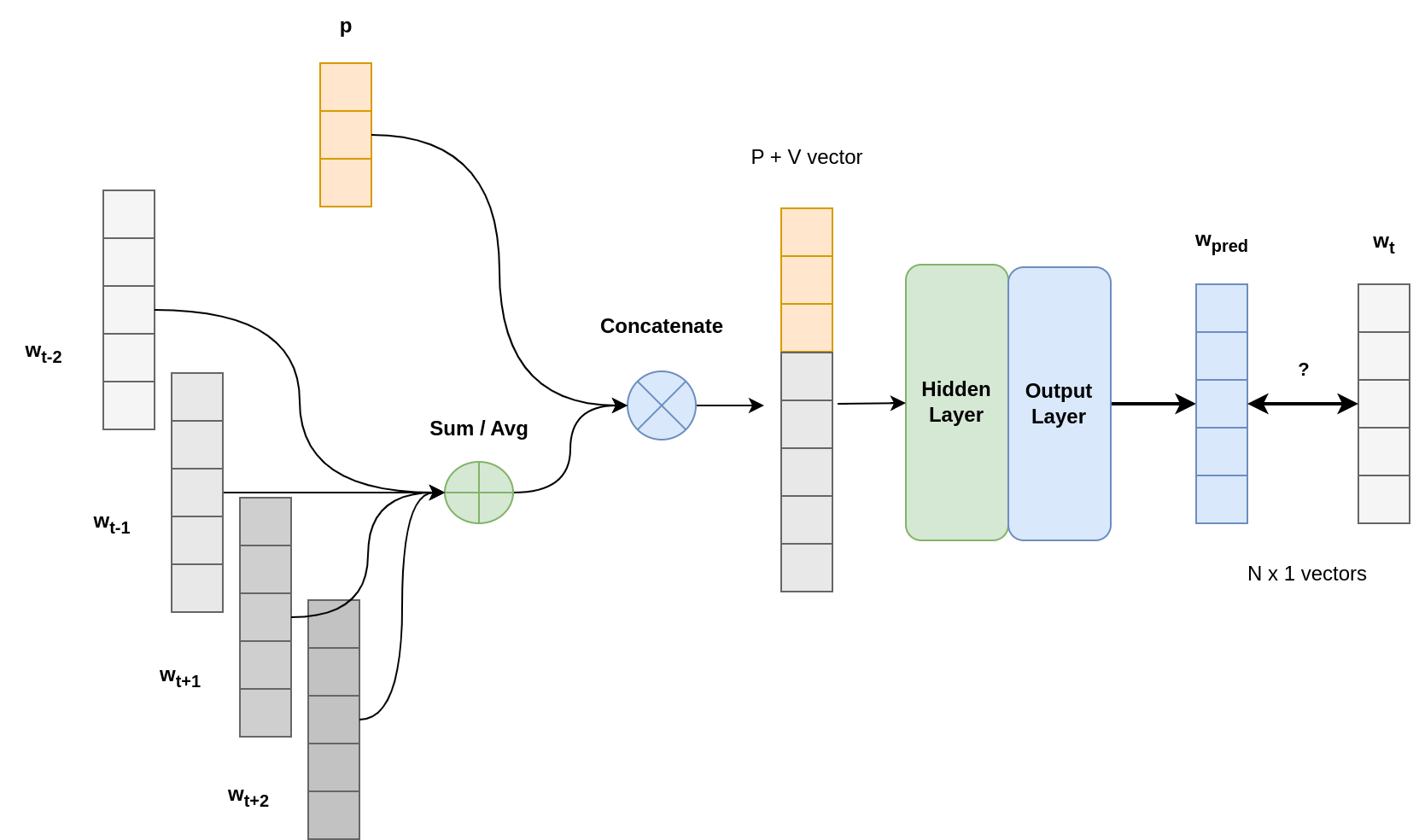
This case is more confortable as the hidden layer is of medium size, and we can extand the context window if necessary.

If you compare this illustration to Word2Vec-CBOW, you can see that here the vector averaging is done before, while in the other figure, it is done after passing through the hidden layer. The thing is: it does not matter. There is no activation function after this layer. Therefore, averaging before or after does not change the outcome !

PV-DBOW

In this configuration, the network receives as input the paragraph vector, and should predict the context words.

Here, this is very similar to the skip-gram model, where the input word is replaced by the paragraph ID.

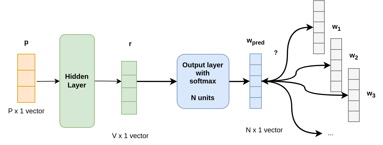
As in skip-gram, the softmax layer outputs word probabilities. Therefore, during inference, this layer returns a weighted list of words.

Usage

While Word2Vec goal is to provide word embedding vectors, the goal of Doc2Vec is to provide document embedding vectors. For all documents of the corpus, we have a representation, thanks to the hidden layer:

PV-DBOW provides document embedding only,
PV-DM provides document embedding and word embedding.

Thanks to these document vectors, we can measure their similarity using the cosine similarity.

For an unseen document, we do not have any corresponding document ID (so no cell allocated in $\mathbf{p}$ vector). The vector is learned “on the fly”: as during training, the algorithm uses the words to learn the paragraph vector. This is as if an additional column was added to all units of the hidden layer. Then, this new weights are updated while all the other are fixed.

GloVe

Global Vectors for Word Representation (2014) ¹⁰ ¹¹

GloVe is similar to Word2Vec as its goal is to find vector representation of words. However, it is not a deep learning model.

In Word2Vec using the CBOW setup, the model is trained by looking at a window of $k$ words around the word of interest to learn its representation. Word2Vec is trained by showing several windows to the model, letting it learn which words go together.

Here, we also look also at a window over the word of interest. However, we collect statistics about word co-occurrences rather than looking at once single window at a time.

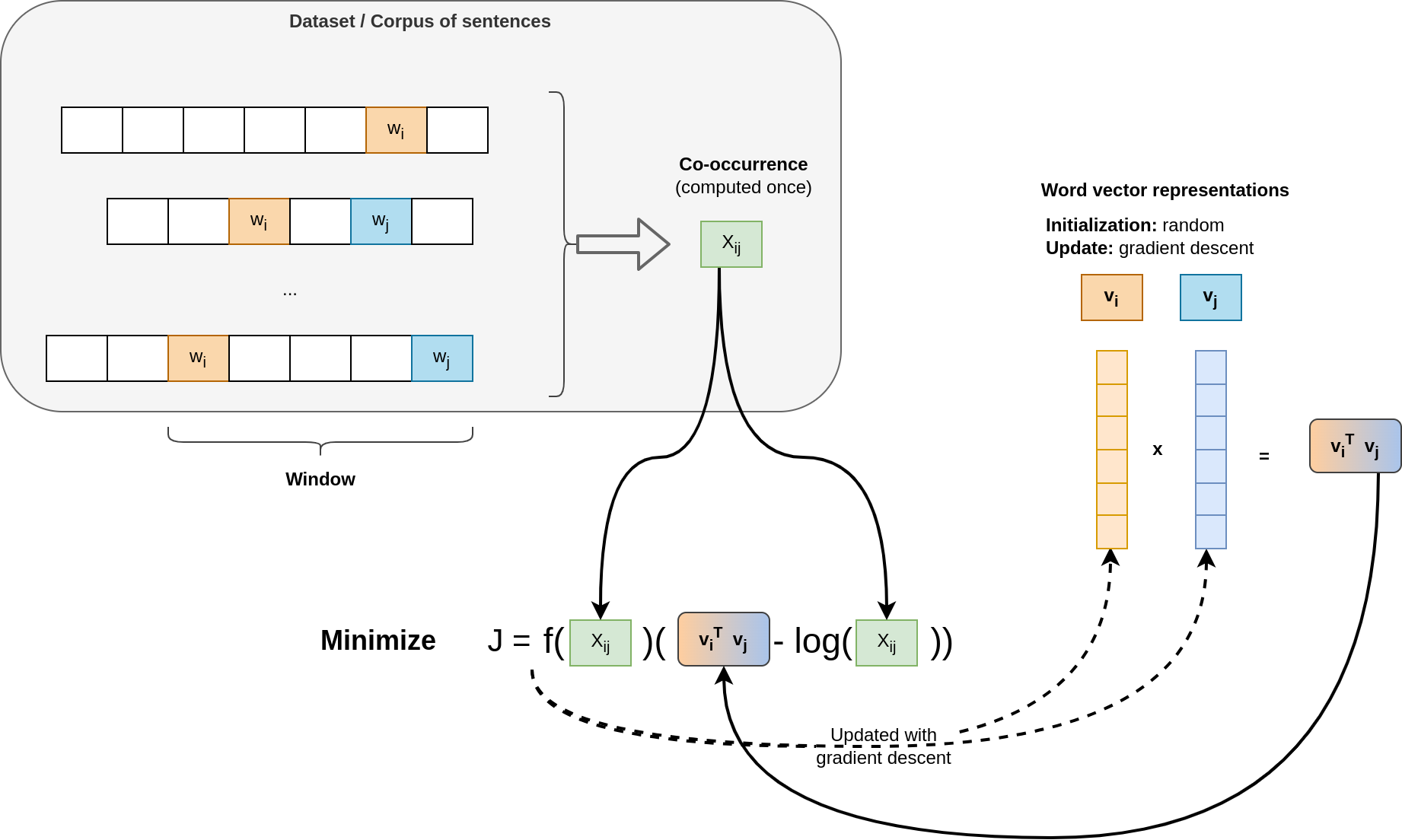
The number of co-occurrences for the word $w_i$ and $w_j$ within a window of finite size is denoted $X_{i,j}$.

Each word $w$ will have a vector representation $\mathbf{v}$ with real weights (in the paper, vectors have a size of $300$).

The goal of this method is to find “good” vector representations, where the product between two word vectors will be a function of their co-occurrence. The cost function is defined as:

\[\hat{J} = \sum_{i,j} f(X_{i,j})(\mathbf{v}_i^T \mathbf{v}_j - \log(X_{ij}))^2\]

Where:

$\mathbf{w}_i$ is the vector representation of word $i$
$f(x) = \min\left(1, \left(\frac{x}{x_{max}}\right)^{\alpha}\right)$ is a function which prevents highly frequent words from having a high contribution. In the paper: $x_{max} = 100$ and $\alpha = 3/4$.

This cost function is optimized thanks to gradient descent with AdaGrad optimizer, and learning over non-zero elements $X_{i,j}$.

Window Weighting

If two words are in the same window but far appart, their contribution should be low. Therefore, the contribution of word $w_j$ to $w_i$ is proportional to $\frac{1}{d}$, where $d$ is the distance between the two words within the window.

Non-Symmetric Version

In the GloVe paper, the initial version pay attention to symmetry. Indeed, in the sentence the cat is cute, cute is after cat. Therefore, there is a need to pay attention to context to the left, and context to the right, as some words preferentially occur after another.

If we want to pay attention to word order, instead of finding a single word vector representation, the algorithm searches two vectors: $\mathbf{w}$ and $\mathbf{\tilde{w}}$. And now, $X_{i, j}$ is computed for $w_i$ appearing before $w_j$, i.e., $X$ is not symmetric anymore.

In this case, the cost function is simply:

\[\hat{J} = \sum_{i,j} f(X_{i,j})(\mathbf{v}_i^T \mathbf{\tilde{v}}_j - \log(X_{ij}))^2\]

Nevertheless, the benefits of asymmetry are limited, as you can always write this is a cute cat.

Seq2Seq

RNN and LSTM have limited capabilities for translation. Indeed, in latin language, the grammar is very similar, so the word order and number is preserved.

In other languages, the structure of a sentence is completely modified, with the verb at the end of the sentence in japanese for instance. These simple networks are unable to remember until the end the verb that should be used.

While RNN and LSTM takes one word at a time, the Seq2Seq model is the first to consider sending a whole sentence to the model. This can be done thanks to progress in hardware and computing power price.

++Slides additional info for training a network

PaperNeurips