Simple Mean-Shift Implementation

Introduction

The Mean Shift ¹ algorithm is quite unknown compared to the \(k\)-means algorithm. Yet, it has the advantage of not requiring the number of clusters to search for.

Table of Content

• Code Samples
  • Notations
  • Move Phase
  • Cluster Identification
• Results
  • Trajectory
  • Density map
• Optimal Code
• Conclusion

How it Works ?

We can decompose the algorithm into two phases:

• the “move” phase;
• the so-called clustering phase.

Code Samples

Notations

We denote \(Y\) the \(n \times d\) vector we want to cluster, where:

• \(n\) is the number of items;
• \(d\) the number of dimensions (in our examples, \(d=2\)).

\(\mathbf{y}_i\) is the \(i\)-est elements of \(Y\), made of \(d\) elements.

Move Phase

During the move phase, we repeat the following operation:

This step update all target elements \(\mathbf{y}_t\) into \(\mathbf{y}_{t+1}\) using a weighted average strategy. Each “reference element” \(\mathbf{y}_i\) is weighted according to a kernel. The kernel gives more weights to reference items that are close to the target element.

The most common kernel is the Gaussian one:

Here, \(\sigma\) is the kernel influence length. A large \(\sigma\) leads to fewer clusters.

However, there are other choices ².

Getting \(\sigma\)

In the simplest mean-shift version, \(\sigma\) is the same for all points. However, it could evolve spatially.

In the case where we want to cluster a \(t\)-SNE embedding, where the density is homogeneous, \(\sigma\) can be computed using the average distance between the \(k\)-nearest neighbors (where in that case, k=perplexity):

from sklearn.neighbors import NearestNeighbors
import numpy as np

def get_sigma(Y, k=30):
    """
    :param Y: Data to be clustered
    :param k: Number of neighbors to consider
    :rparam: sigma / kernel characteristic length
    """
    md = NearestNeighbors(n_neighbors=k+1).fit(Y)
    NN = md.kneighbors(Y)[1][:, 1:] # n x k int array

    return np.median(np.sqrt(((Y[NN] - Y[:, np.newaxis])**2).sum(axis=2)).mean(axis=1))

Displacement Loop

The Mean-Shift is very simple to implement. We only need a few lines of code.

import numpy as np

def mean_shift_loop(Y, sig=1.0, n_steps=20):
    """MeanShift implementation

    :param Y: Vector to update
    :param sig: standard deviation, homogeneous to distance
    :param n_steps: number of loop to perform
    :rparam: Array of shape of Y
    """

    # Exponential kernel definition
    fx = lambda d2:  np.exp(- d2 / (2 * sig**2))

    # Move loop
    Yi = Y.copy()
    for _ in range(n_steps):
        Di = fx(((Yi[:, np.newaxis] - Y)**2).sum(axis=2))
        Di = (Di.T / Di.sum(axis=1)).T # Norm to 1

        Yi = np.array([Y[:, d] @ Di.T for d in range(len(Yi[0]))]).T

    return Yi

Cluster Identification

Now, we need to gather items into clusters. For this step, we apply the following rule:

If the distance between two elements is less than \(\epsilon\), then they belong to the same cluster.

The simple thing is to set \(\epsilon = \sigma\), as the clusters should be distant enough.

def cluster_component(Y, eps):
    """Identify clusters

    :param Y: Vector to cluster
    :param d: maximal distance between two items in a cluster
    :rparam: (groups, assignement)
    """
    n = len(Y)

    # We record for each groups elements that are in
    dic_gp = dict([(i, [i]) for i in range(n)])
    # We record for each item the group it belongs to
    dic_ID = dict([(i, i) for i in range(n)])

    # Loop
    for idx, y in enumerate(Y):
        # We identify neigbors in the radius
        locs = np.where(np.sqrt(((Y - y)**2).sum(axis=1)) < eps)[0]

        # Group that will replace all
        GID = dic_ID[idx]

        # Gather all elements that belongs to connected clusters
        all_gp = set([dic_ID[x] for x in locs])
        all_elements = []
        for gid in all_gp:
            all_elements.extend(dic_gp[gid])
            del(dic_gp[gid])

        # Gather all elements in a single group
        dic_gp[GID] = all_elements
        for c in all_elements:
            dic_ID[c] = GID

    # Create assignement vector.
    arr = np.zeros(n)
    for idx, gp in enumerate(dic_gp.values()):
        arr[gp] = idx

    return list(dic_gp.values()), arr

Results

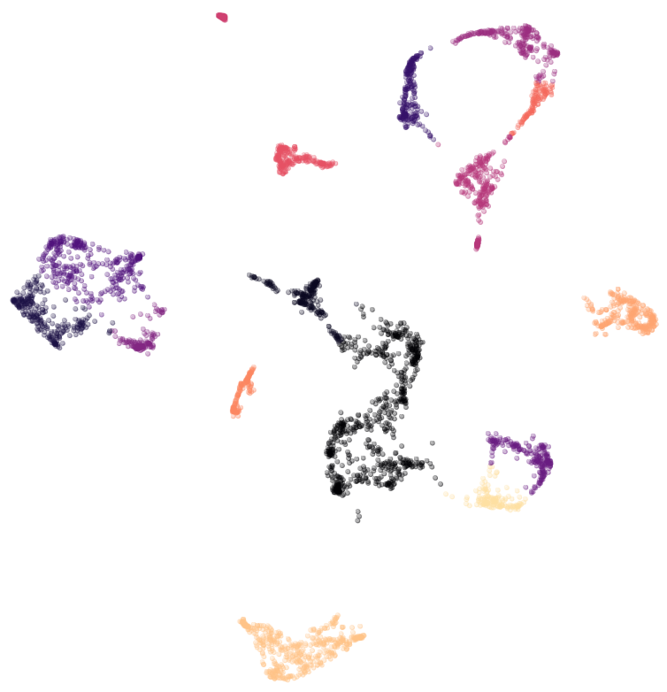
We have made several Bokeh plots to illustrate the mean-shift clustering process.

Trajectory

In the figure bellow, points are colored according to the cluster found using the MS algorithm (there is no ground truth)

Use the slider slice to see the different iteration steps.

You can zoom in and increase the size of the dots to better visualize the displacement.

You can see how quick the elements aggregate into “snakes”, and then it takes a little more time to converge to local spots.

(Note: here, knn=120)

Density map

Before any iteration steps, we can compute where the cluster centers would be. For that, we can create a density map using the defined kernel:

GRAIN = 400 # Resolution of the map

x0, y0 = Y.min(axis=0)
x1, y1 = Y.max(axis=0)


xx = np.linspace(x0, x1, GRAIN)
yy = np.linspace(y0, y1, GRAIN)

XX, YY = np.meshgrid(xx, yy)

# Kernel definition
fx = lambda d2:  np.exp(- d2 / (2*sig**2))

# Loop to measure density
D = np.zeros(XX.shape)
for x, y in Y:
    D += fx((XX - x)**2 + (YY - y)**2)

If we put the resulting image in background, we get the following plot:

What you can see is that points converge towards very specific location, which are called “mode”. They are maximum of probability density, and you always reach them if you follow the gradient.

Thanks to this map, you can segment into areas the space, and guess where each item will go.

Here is another example with a smaller bandwidth \(\sigma\) (knn=60)

Optimal Code

The previous code is very slow on large dataset. The problem is that we compute the distance between all pairs. However, the kernel would give a weight of \(0\) to elements that are far away. Therefore, when you cluster around 10,000 points, less than 100 are useful at each step (though, it depends on sigma).

To prevent from computing distances between irrelevant pairs of items, we can optimize it by computing distance only between the target item and its nearest neighbors.

from sklearn.neighbors import NearestNeighbors

def mean_shift_opti(Y, sig=1., knn=30, n_steps=50):
    """Fasten Meanshift using nearest neighbors

    :param Y: points to cluster
    :param sig: sigma found during previous step
    :param knn: better to use x 2 (from sigma)
    """

    # Model to get quick access to nearest neighbors
    md = NearestNeighbors(n_neighbors=knn).fit(Y0)

    # Gaussian Kernel definition
    fx = lambda d2:  np.exp(- d2/(2*sig**2))

    Yi = Y.copy()
    for _ in range(n_steps):
        neigh = md.kneighbors(Yi)[1]
        Di = fx(((Yi[:, np.newaxis] - Y[neigh])**2).sum(axis=2))
        Di = (Di.T / Di.sum(axis=1)).T # Norm to 1
        # Perform the update
        Yj = np.array([(Y[neigh][:,:, d] * Di).sum(axis=1) for d in range(len(Yi[0]))]).T

        Yi = Yj

    return Yi

For a 2D dataset of 8,000 items, the first code runs in 150 seconds while the second in 10 seconds.

For the same \(\sigma\) and n_steps, we can compare the two clustering outcomes using the NMI (Normalized Mutual Information), to see if they lead to the same result.. We get 98.45 % which is a good similarity result.

(OK, this small experiment has been done on one trial, this is not significative, however you can try it yourself)

Conclusion

In this article, we described how the mean-shift algorithm works, and provide a simple python implementation. We provide also an optimal version which runs much faster on large datasets.

Sources

>> You can subscribe to my mailing list here for a monthly update. <<