Co-Embedding - Visualisation of a bipartite graph

Introduction

While most algorithms focus on structured data (data that can be represented as a table), many problems are graphs. Social networks, interactions, publications, blog posts, … One particular data structure is bipartite graph: this is a graph (i.e., a set of nodes connected by edges), where there are two kinds of nodes and where connections exist only between nodes of two different kinds.

To the non-specialist, this might be weird, but this is exactly the topic of recommander systems: there are users who read books, or who buy products, or like post. We do not know the users’ relationship, if they are friends or not, part of the same community, but knowing their taste, we want to discover their relationships.

A general problem with graphs is their representation. Tabular data can be easily represented by selecting 2 or 3 dimensions, and plotting the items, or performing PCA to compress components. For graph, there is no “dimension”, and visualization is difficult.

Here, we describe an embedding strategy, where we exploit relationships

Table of Content

• Introduction
• Usual Processing
  • From Graph to Table
  • Measuring similarity
  • Neighborhood Analysis
• Measuring similarity in a sparse environment
  • Pruning Links
  • Schematic view of the process
  • Measuring similarity on an embedding
  • Comparing vectors
  • Code structure
  • Isolating Cluster
• Results
  • Visualization
  • Evaluation
• Conclusion
• Sources

Usual Processing

From Graph to Tabular Data

A graph is a data structure made of nodes and edges. Nodes represent entities while edges represent relationships between entities.

In the graph family, there are bipartite graphs, which are graphs where there are two kinds of nodes, and edges can only connect two nodes of different kind. This type of graph is very frequent in the world of recommender systems. For instance, the first type of node would be the users’ node, while the second kind is the books’ node. There would be a relationship between a book and a user if the user has read the given book.

Let’s take an example with three users \(u_a, u_b, u_c\), and five books, \(b_1, b_2, b_3, b_4, b_5\), and suppose that:

• user a has read book 1, book 2, and book 3,
• user b has read book 4 and book 5,
• user c has read book 2, book 3, and book 4,

This is the bipartite graph representation:

And an “optimal” graph encoding would be:

{
  "ua": ["b1", "b2", "b3"],
  "ub": ["b4", "b5"],
  "uc": ["b2", "b3", "b4"]
}

However, this representation is not very convenient. To compute quantities, it is preferable to have arrays where each dimension represents the same thing. In the case of a bipartite graph, we can convert the graph into a binary matrix, where:

• A row represents one user
• A column represent one book
• We put a \(1\) on \((r_u, c_b)\) if the user $u$ has read the book $b$, $0$ otherwise.

Therefore, an alternative representation would be:

Similarity

In recommender systems, there are several main questions:

• “How do I measure similarity between elements?”, i.e., similarity between users, or similarity between books.
• “How do I find new books that the user may like?”

Both questions require to define a similarity function, or a way to score a pair \((u_i, u_j)\), \((b_i, b_j)\) or \((u, b)\).

For two items of the same kind, the most basic approach is to measure the cosine similarity between the two vectors representing the items. When comparing two users \(u_1\) and \(u_2\) with respective vector \(r_{u_1}\) and \(r_{u_2}\), the cosine similarity is computed as:

This works well when the binary matrix is not too sparse, and that items are homogeneously distributed, which does not happen frequently in real life:

• There are always items/books that are very popular (Harry Poter), while many are almost unknown (Comment parler des livres que l’on n’a pas lus ?¹),
• There are always users that are heavy readers, while many users read very few books per year.

For instance, if I look at the Lastfm dataset ² subset, where we have music names associated with keywords, we obtain this matrix:

This is not a joke ! There are very thin horizontal lines which correspond to tags which occur in many musics. Unsurprisingly, the three top keywords are rock, pop and alternative.

If we plot the number of occurrences per tag, and sort them by decreasing order, we get this curve:

This is what we call a power-law distribution: a few items occur very frequently while the rest almost never.

To get a better view, we simply need to move to the log scale:

If we do the same analysis for music, the behavior is less pronounced, as the maximal number of tags per music is limited:

(Here, the floor is at 3 because we performed some filtering to remove items with less than 3 occurrences).

In these conditions, it is very difficult to find relationships between musics:

• Many items will share the rock keyword, however this is not discriminative at all.
• As you can see, there are many musics where there are 3 keywords. For those, it is difficult to do something with.
• For the rest, the overlap is very small: assuming we consider only music with at least 5 tags (here, on average 6.2 tags/music), we have around 500 keywords. The probability that there is an overlap (forgetting about power law) is very low …

This approach, where we only consider the direct links between a music and its tags, is dead-end.

Neighborhood Analysis

If the direct neighborhood is insufficient to describe an item, we can explore the neighborhood to add context and improve the overlap between vectors.

To do that, we exploit the graph: we start from a book, look at users who have read this book, and next look at the books those users have read, to obtain a new group of users, and explore recursively the space:

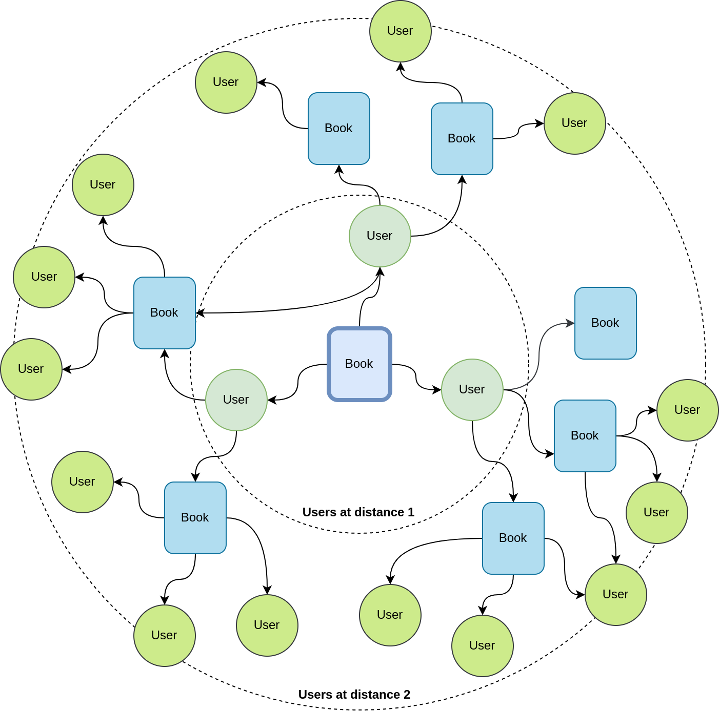
The question is “when do you stop the exploration ?” Do you stop at distance \(2\) ? \(3\) ? Or more ? Knowing that on average, a user read \(B\) books, and a book is read by \(K\) users, the number of books grows as \((KB)^d\), where \(d\) is the distance, which quickly explode to very large values. And here, you begin to think to the opposite problem: Which information is relevant? How do you filter that ?

When doing the exploration, we need to weight down:

• distant items, as the more distant they are, the less relevant
• children of a node with many links: If a node is connected to many links (e.g., Harry Poter), it is unlikely to provide strong evidence.

The random walk algorithm does exactly this weighting. Nevertheless, you still need to decide when to stop the exploration.

How to Measure Similarity in a Sparse Environment

We wanted to answer this question with something different from the random walk, and more adapted to bipartite graphs.

Idea: Pruning Links

In a graph, there are relationships that are relevant, and others that are not. Sometimes, someone has read a book, but he did not like it. How do we know ? Unless there is a scoring system, we never know. Therefore, we wanted to explore this question of pruning weak links.

To prune a link, we need evidence that two nodes do not match correctly. For this, we need to analyze information from the neighborhood of these two nodes. Rather than making a voting system, we propose to break link through projection.

When projecting data in a low dimensional space, we face the crowding problem, where it is impossible to preserve all relationships. At least, the projection should preserve the most relevant relationships. However, our initial problem which is to prune weak links is equivalent to finding strong relationships. We fall into the chicken-egg problem!

Here comes the second part of our idea: as in gradient descent or KMeans, we never reach the solution at the first step. We need several iterations to reach an optimal solution.

And the last part of the idea is to measure the items’ similarity on the embedding, to exploit the knowledge extracted from the projection.

We will detail the complete idea in the following paragraphs.

Processing

Starting point:

1. Compute the similarity between books, and similarity between users using the binary matrix, using the cosine similarity.
2. Create two first embeddings (one for books, one for users), using SVD

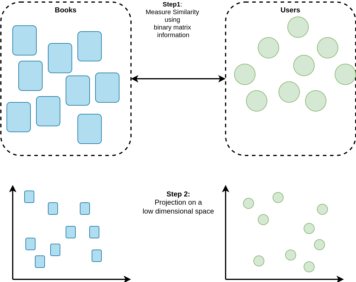
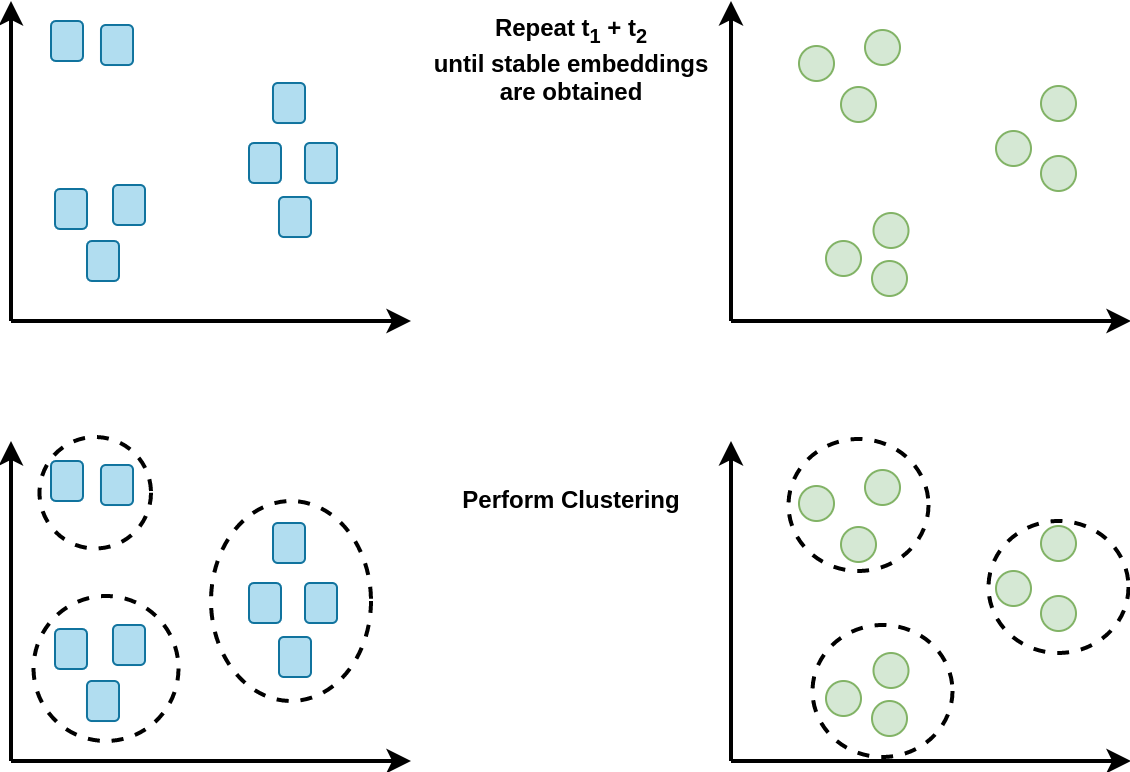
Now, repeat several times the two following steps:

1. Measure the book similarity using the user embedding (and inversely)
2. Update the two embeddings using the new similarity information

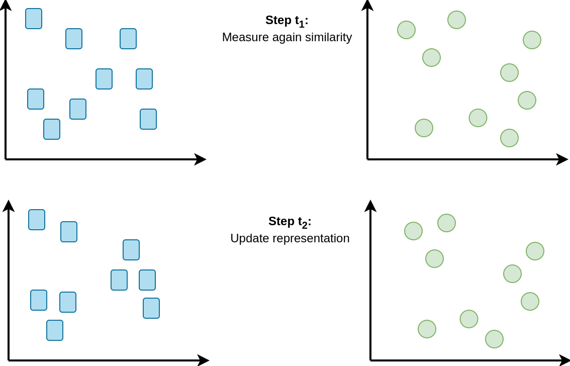
Then, when the embeddings do not change that much anymore, perform clustering.

How to Measure Items Similarity on an Embedding

Depending on which algorithm is used, properties of the embedding are differents.

• For the first embeddings, we use SVD which tries to extract eigen vectors.
• For the iterations, we use \(t\)-SNE because it tries to preserve strong local relationships and provides very nice visualization results, which are also easy to cluster ³.

\(t\)-SNE uses two kernels: a \(t\)-student kernel and a Gaussian one. Therefore, we use a Gaussian kernel to retrieve the neighborhood information.

Suppose a user has read two books, b1 and b2. To measure relationships between users, we will update the binary vector of this user using the books’ neighborhood. In the following example, b3 will contribute because it is in the neighborhood of b1, as well as b4 and b5 in the neighborhood of b2.

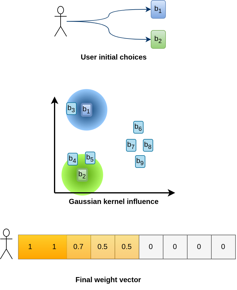
We can measure the contribution of b4 relatively to b2 as:

where:

• \(K_2\) is a normalization constant ensuring that \(\sum_{b \in \mathcal{B}} C(b \| b_2) = 1\), which prevents nodes in a very dense neighborhood from contributing more than nodes in a less dense neighborhood,
• \(\sigma\) is the radius of influence, which governs how many neighbors should contribute. The value is fixed for all nodes.

Because b4 is too far from b1, its contribution is \(C(b_4 \| b_1) \approx 0\).

With this idea, we create a vector \(\mathbf{v}\) where:

\(D_i\) is a second normalization constant which ensures that \(\sum_i v_i = 1\), i.e., this vector is analog to a probability distribution over the embedding space.

Measure Similarity Between Embedding Vectors

The cosine similarity leads to very small scores when the arrays are large and the overlap small. This prevents us from differentiating strong from weak relationships.

Instead, we propose the use of the symmetric Kullback-Leibler divergence:

And:

where \(\mathcal{v}\) and \(\mathcal{w}\) are both vectors representing users (or books).

The divergence, which is a distance between probability distribution can be considered as the distance between the elements (between the books, or between the users).

Note: This is not the Jensen-Shannon divergence: here, there is a large penalty if one vector does not overlap the other.

Piece of Code

We just illustrate the process to update the embeddings:

from sklearn.manifold import TSNE

[...]

for _ in range(10):
    # Sigmas is a parameter to adjust radius to the current embedding
    # k is the number of neighbors to consider
    sigma_b = get_sigma(Yb, k)

    # Compute user vectors using book embeddings
    V = get_gauss(M, Yb, sigma_b)


    # Compute distances
    Du = KL_sym(V, V)

    # Update the embedding
    Yu = TSNE(init=Yu, metric="precomputed").fit_transform(Du)

    # Same process but the roles are reversed.
    sigma_u = get_sigma(Yu, k)
    W = get_gauss(M.T, Yu, sigma_u)
    Db = KL_sym(W, W)
    Yb = TSNE(init=Yb, metric="precomputed").fit_transform(Db)

Getting Clusters

The \(t\)-SNE algorithm often led to patterns very easy to cluster. As we do not know the number of clusters to expect, we selected the Mean-Shift algorithm ⁴, where only a bandwidth parameter \(\sigma\) is necessary to adjust the Gaussian Kernel. This parameter is estimated over the embedding.

Results

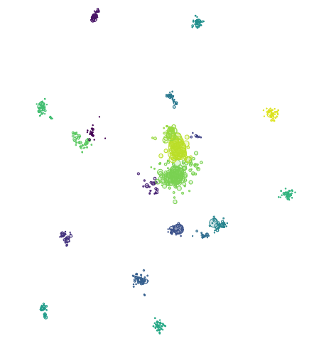
Visualization

Below is a bokeh interface to interact with the results and visualize the updating process.

The left plot corresponds to music_title::artist, while the right one to associated tags (where you may see artists’ name).

The Mean-Shift algorithm is run on the last slice, and the coloring is applied to all previous locations to follow the migration process.

How you can interact the following ways:

• You can change the slice ID (i.e., see the previous embedding)
• You can change the point size (more convenient if you want to use the hover)
• There is a “lasso tool” which enable to get the list of elements selected

Evaluation

We proposed to evaluate the cluster relevance using the following task.

The goal is to retrieve a book given the list of users who have read this book.

Suppose all books of a given cluster are stored in a dedicated server, this for all clusters on different servers.

This is for efficiency. Instead of searching one book in a database with \(n\) entries, we would search in a database with only \(\frac{n}{k}\) entries, which will speed up the search process. The real goal would be to retrieve the server where the book is stored.

Using the user clusters, we compress the book representation by aggregating the users by categories, transforming \(\mathbb{v}(b)\) into \(\mathbb{v}'(b)\):

To obtain a book cluster descriptor, we average over all books of this cluster, and get \(\mathbb{\bar{v}}\):

Now, we get a query which is book vector, i.e., the 0/1 represents the users having read this book. This vector is compressed using the user clusters.

To decide to which server to root the query, we measure the KL divergence between all cluster prototypes:

The book cluster with the lowest divergence is selected. Numerical results and comparison with other methods are detailed in the original paper ⁵.

What is the Purpose ?

Ok, we were able to represent our graph into a 2D space. What can we do we that ?

First of all, profiling, which is the analysis of the clusters. You have groups of similar music, similar books, similar tags. Knowing they belong to the same group enable to compress the representation and fasten the similarity search.

Next, you can study relationships between clusters. Here, most clusters do not touch each other. Therefore, it is impossible to infer something about their relationships (this is a property of \(t\)-SNE). However, it does not mean they don’t share anything: For clusters of users, they may share part of their book nodes, but not all. Studying the relationships between cluster enable to recommend new elements.

Conclusion

We developed a new way to measure similarity for recommender systems using embeddings. When representing items in a low dimensional space, weak relationships are broken. We recovered strong relationships by applying a Gaussian kernel around all elements and repeated the (embed)-(similarity measurement) until stable clusters were obtained. The clusters were easily recovered using the Mean-Shift algorithms, and the coherence of the cluster was strong.

Sources

>> You can subscribe to my mailing list here for a monthly update. <<