Napoleon X Challenge - Part III - Predicting Accurately Data

Introduction
This is the third post of the series about Napoleon X Challenge.
- Part I is the data analysis part, where we discovered how to put stuff together.
- Part II is the time series disambiguation part. We were able to partially find which crypto-asset corresponds to which time series.
Part III(this one) explains how we obtained a very good prediction accuracy using what we learned inPart Iand a simple linear regression model.
Last post is a presentation made at Collège de France at the end of the challenge.
Reminder
As a reminder of the dataset and the prediction task:
- We have time series representing asset returns for 21 days for the first 23 hours.
- Each cluster is made of several assets
- Assets have a relative ID within a cluster.
- A cluster lives for three weeks
- The goal is to predict the average return for all 21 days for the 24th hour for the cluster.
What we learned in Post 1 is:
- We were able to find assets in the dataset which represented the same crypto-asset
- We were able to find the relative date, relatively to the earliest chunk.
- The dataset is recorded over 215 weeks.
In Post 2, we understood what is the meaning of md and were able to identify the name of the crypto-asset (e.g. ethereum, litecoin, …).
Post 2 doesn’t really help, but confirms that we were right about asset matching.
Predicting Average Return Accurately
In post 1, we saw that assets are correlated, or more specifically, they are impacted by a global trend.
Therefore, they more or less go in the same direction.
We exploited this fact to fill the test sheet in post 1, filling the value with the average given the current week-day.
Here, we will try to be more accurate by exploiting assets of clusters.
How Much is Overlapping ?
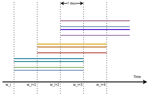
As a cluster exists for three weeks, and a new set of clusters is issued every week, it means that for a given week, we have three generation of clusters at the same time. The following figure illustrate the process with:
4clusters generated at weekw_i,3clusters generated at weekw_i+1,4clusters generated at weekw_i+2.

Which means that if we want to infer something about returns for a given day occurring in week w_i+2, we have information about 11 clusters.
Clusters VS Assets
We have clusters and we have assets. Fortunately, the overlap between train and test assets is relatively large.
If we take as an example week 12, there are 8 clusters:
4train clusters4test clusters
And for week 11, there are 4 clusters, and 8 for week 10.
Therefore, we have 16 clusters to help us predicting returns for the test clusters.
Now, if we look at assets, among these 16 clusters, there are 120 unique assets.
For the 4 test clusters, there are only 70.
Among these 70, 69 are shared with the train clusters.
Because the number of clusters is much smaller than the number of assets, it is impossible to recover the exact value of each asset. However, we can identity the group trend, which is useful enough.
We can represent assets as a binary matrix, where each row represents a cluster, and each column an asset.
For training, we get the binary matrix:
For testing, we get the binary matrix:
Prediction with Linear Regression
We have a set of \(c\) clusters, each made of a given set of assets, represented by the matrix \(M \in \{0, 1\}^{c \times a}\). The average return of the cluster is \(\mathbf{y} \in \mathcal{R}^{c}\).
We want to find \(\mathbf{w} \in \mathbb{R}^{a}\) such as:
\[\arg\min_Y \|\hat{M} \mathbf{w} - \mathbf{y}\|^2\]where \(\hat{M_{i, j}} = \frac{M_{i,j}}{\sum_k M_{i, k}}\) is the matrix \(M\) row-normalized. This normalization is necessary because \(\mathbf{y}\) is the average return. Therefore, the more assets there are, the less each individually contributes.
Coding
Coding what we presented above is easy.
sklearn and numpy are needed to not reinvent the wheel.
The only difficulty is to recover predicted values for the different weeks without getting wrong on the index.
Otherwise, when the binary matrices are isolated and average returns of train clusters extracted, the game is easy:
W  = M.sum(axis=1) # M is the train binary matrix
W1 = M1.sum(axis=1) # M1 is the test binary matrix
# We normalize both, because what we measure is the average return
M = (M.T / W).T
M1 = (M1.T / W1).T

for i in range(7): # For each day of the week
    md = LinearRegression()
    md.fit(M, Y_train[:, i]) # Y_train is the average return for each train cluster
    y_test_i = md.predict(M1) # This is the estimated average return for the test clusters.
    # + Other operations to store `y_test_i` in the correct location of the submission sheet.
Harmonization
The linear regression is possible and effective if:
- the number of train clusters is sufficiently large
- the assets of test and train clusters overlap
These are hypothesis, and are not always fulfilled. Because we have 1463 train clusters and 627 test clusters, the probability that the first hypothesis is not verified is low. However, for the second, it happens that the overlap is too small to be accurate.
In that case, we remember that crypto-assets are affected by the main global trend.
Therefore, we go back with prediction made in post 1 using the average when we do not have enough information about assets.
Getting the average
In our code, we have reshaped the dataset in a more convenient form.
Instead of having rows with one asset and one day of data,
we have DX where each row represents one asset over 21 days in its cluster, with columns:
- 503 return columns (
21 x 24 - 1, with 24 hours filled with0.) - Cluster ID
- Asset ID with this cluster
mdandbctime, which corresponds to the starting week of the clusterassignment, which is the global assetID, which is independent of time.
With this format, it is easier to extract average return for each day.
# Initialization
dic_mean_list = {}
for tx in range(0, 216):
    for i in range(7):
        dic_mean_list[tx*7+i] = []

for tx in range(0, 216):
    S = set(DX[DX.time == tx].cluster)
    S = list(filter(lambda x: x <= 1463, S))
    for c in S:
        for i in range(21):
            y = data_y.loc[c*21 + i].values[0] # Y Train sheet
            dic_mean_list[tx*7+i].append(y)
Filling Extreme Values
We just have to find where are located extreme values, and replace them with the mean return of train clusters.
vlim = 0.1 # Threshold for correction
for i in np.where((data_y_pred.values > vlim) | (data_y_pred.values < -vlim))[0]:
    sample_id = data_y_pred.index[i] # Get the sample ID
    cls = sample_id // 21 # Extract corresponding cluster
    day = sample_id % 21 # Extract day
    # DX is a dataframe where for each cluster, we have a `time` column corresponding to the starting week.
    t0 = int(DX[DX.cluster == cls].time.values[0] * 7 + day)
    vr = np.mean(dic_mean_list[t0]) # Averaging
    data_y_pred.loc[sample_id] = vr
In our case, we found 250 extreme values, which is very small compared to the 13133 sample ID.
However, because of their amplitude, they would affect the evaluation score.
Checking Distribution
Now that we have filled the blanks, we can check if the train and test sets have a similar returns distribution.
When looking at it, we still get a Cauchy distribution, with a negligible difference.
Submitting
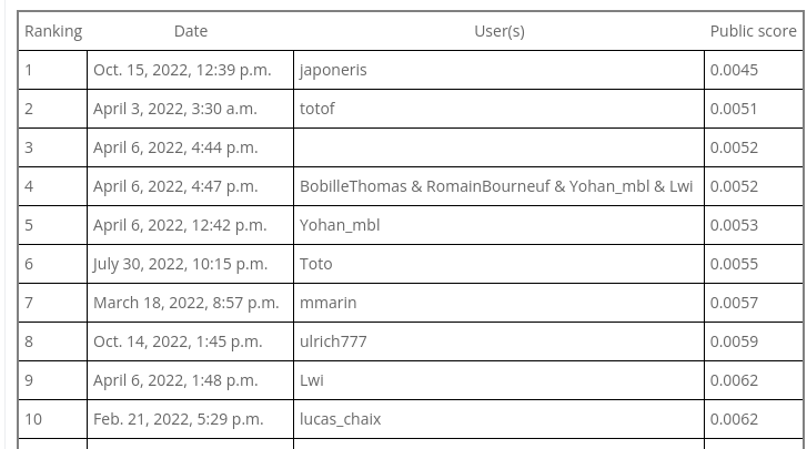
We reduced our MSE from 0.0061 to 0.0045, and moved from rank 7 to rank 1.
1st rank, without any complicated algorithms. Just pure logic and basic things.

Enjoy !
Link to Part IV
>> You can subscribe to my mailing list here for a monthly update. <<


